Orthtree Algorithm

Orthtree is a discretization algorithm for 3D and 2D domains that uses a spacing function (for example BoundaryLayerSpacing) to adapt point density:

• finer near walls/boundaries,

• coarser in the bulk interior.

The name is the dimension-agnostic term for -ary spatial subdivision trees (as in CGAL's Quadtrees, Octrees, and Orthtrees): the algorithm guides its fill with a SpatialTree — an octree in 3D, a quadtree in 2D.

This is useful for CFD and boundary-layer-dominated meshless simulations where you need high resolution close to surfaces without over-resolving the full volume.

Basic Usage

using WhatsThePoint
using Unitful: m

mesh = import_mesh("model.stl", m)
boundary = PointBoundary(mesh)

spacing = BoundaryLayerSpacing(
    points(boundary);
    at_wall=0.6m,
    bulk=4.0m,
    layer_thickness=8.0m,
)

alg = Orthtree(mesh)
cloud = discretize(boundary, spacing; alg)   # max_points auto-estimated

The algorithm is designed primarily for 3D geometries — its production home is volume discretization of surface meshes. A 2D counterpart is available and behaves identically (see 2D Domains below); the figures on this page use a 2D domain because the mechanics are easier to see in the plane.

The first stage is the spacing-driven node tree (octree in 3D, quadtree in 2D): boxes subdivide until their size satisfies h_box ≤ alpha · h(x), so the tree is fine where the prescribed spacing is fine — here, near the wall:

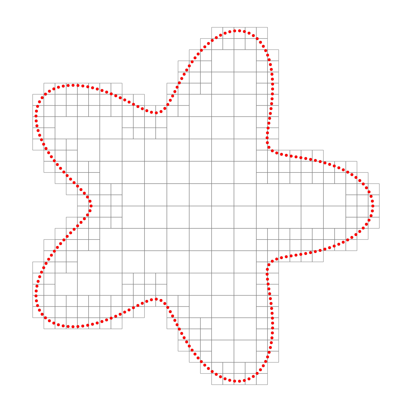
The node quadtree over a starfish boundary (red points). With a graded BoundaryLayerSpacing, boxes refine toward the wall; the tree only keeps boxes that can host domain points.

Bridson Placement (default)

The default placement mode, :bridson, runs a single global advancing-front Poisson-disk pass (Bridson 2007) graded to the spacing field h(x): every generated point keeps a distance of at least min(rᵢ, rⱼ) with r = bridson_factor·h(x) from every other point — including the boundary seeds — by construction. The front saturates on its own, so no refinement or repulsion pass is needed afterward, and max_points acts as a non-truncating cap (auto-estimated from the spacing integral when unset; a warning fires if a hand-set cap truncates the front).

With max_growth > 0, the prescribed spacing is replaced by its gradient-limited (Lipschitz) envelope before sampling, so steep boundary layers transition smoothly instead of jumping — 0.1–0.2 matches typical CFD growth ratios of 1.1–1.2.

A too-coarse spacing (one the domain cannot host an interior at) is clamped with a loud warning instead of silently producing an empty cloud; run suggest_spacing first to pick a viable spacing deliberately.

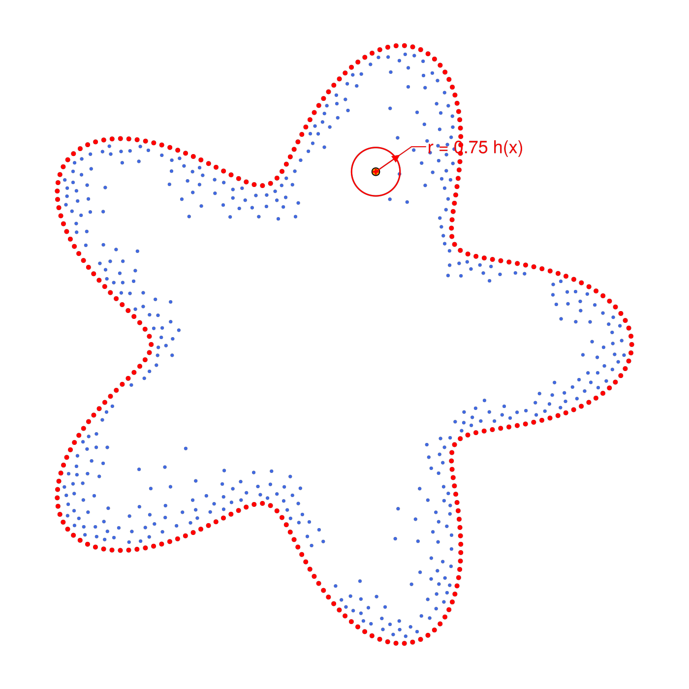
Bridson placement is dart throwing: candidate points are proposed around the advancing front and accepted only if they pass a set of rules. The decisive one is spacing satisfaction — the candidate must have no neighbor within its spacing radius r = bridson_factor · h(x) (a disk in 2D, a sphere in 3D). The encircled point is an accepted dart: its disk contains no other point, by construction.

2D Domains

The same algorithm runs on 2D boundaries — and is the 2D default, so discretize(bnd, spacing) already uses it. A SegmentQuadtree indexes the segments of one or more closed loops, and the node tree, leaf classification, and Bridson front work exactly as in 3D. A boundary is just an ordered loop of points — build it, and the familiar three lines apply (passing alg explicitly here only to show where the geometry index comes from):

using WhatsThePoint
using Unitful: m

# Starfish boundary: sample a parametric curve at ~equal arc length
r(θ) = 1 + 0.3 * cos(5θ)
θs = range(0, 2π; length = 20_000)
xs, ys = r.(θs) .* cos.(θs), r.(θs) .* sin.(θs)
arclen = cumsum(hypot.(diff(xs), diff(ys)))
targets = range(0, arclen[end]; length = 259)[1:(end - 1)]
idx = [searchsortedfirst(arclen, t) for t in targets]
pts = Point.(collect(zip(xs[idx], ys[idx])))

bnd = PointBoundary(pts)                # ordered loop of boundary points
spacing = BoundaryLayerSpacing(
    points(bnd);
    at_wall = 0.035m, bulk = 0.14m, layer_thickness = 0.35m,
)
alg = Orthtree(bnd; spacing)              # SegmentQuadtree geometry index
cloud = discretize(bnd, spacing; alg)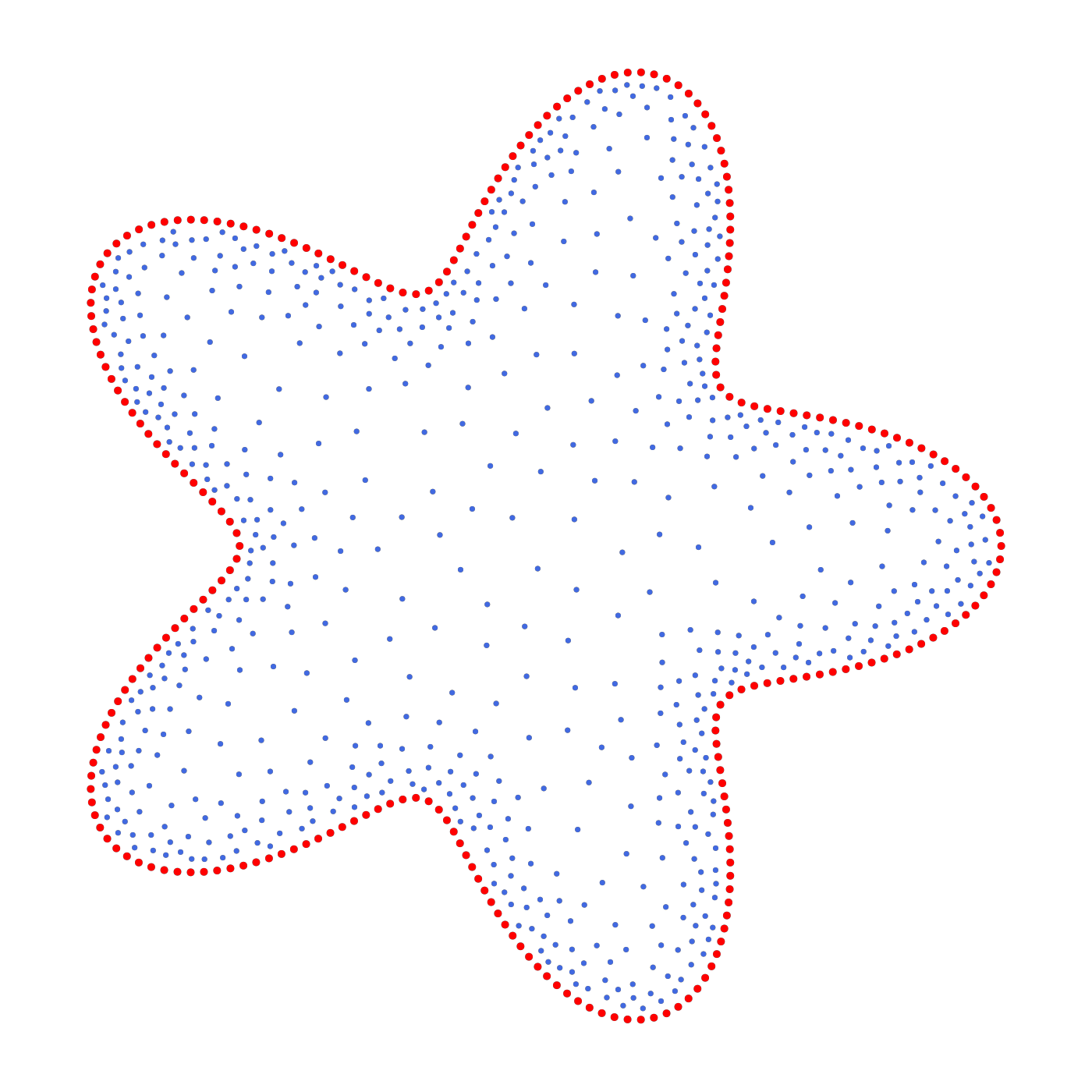

The finished cloud: boundary points (red) and the graded interior fill (blue) — dense in the wall layer, coarse in the core, Poisson-disk quality throughout.

Passing multiple surfaces (loops) in the PointBoundary describes multiply-connected domains: outer boundary plus holes. Loop orientation does not matter — it is normalized automatically.

Parameters

The constructor supports the same orthtree controls used elsewhere, plus placement options for candidate generation:

• orthtree refinement controls (tolerance_relative, min_ratio, node_min_ratio, alpha)

• placement mode (:bridson default, or per-leaf :random, :jittered, :lattice)

• Bridson disk radius relative to spacing (bridson_factor, default 0.75)

• gradient-limited spacing (max_growth, default 0 = off)

• boundary leaf oversampling (boundary_oversampling, per-leaf modes only)

• orientation and safety checks (verify_orientation, etc.)

See Orthtree and BoundaryLayerSpacing in the API reference for the exact signatures.

Included Example Scripts

Full runnable examples are included in this repository:

• examples/octree_boundary_layer.jl (3D)

• examples/octree_quadtree_2d.jl (2D)

The 3D script demonstrates: 2. probing the geometry with suggest_spacing,

3. Poisson-disk boundary sampling and a steep gradient-limited BoundaryLayerSpacing,

4. running Orthtree (Bridson placement, auto point budget),

5. checking quality (spacing_fidelity_metrics, metrics) and rendering cross-section PNGs with CairoMakie,

6. writing a ParaView .vtu via export_vtk.

The 2D script builds the starfish domain above and renders the three figures shown on this page (node quadtree, Bridson dart, finished cloud).

Notes

• Orthtree supports 3D boundaries (from meshes) and 2D boundaries (closed loops of ordered points).

• For uniform spacing, SlakKosec is a good alternative in 3D.

• If your model scale changes significantly, tune at_wall, bulk, and layer_thickness in physical units.