Discretization

Volume discretization generates interior points from a boundary surface. This is typically the second step in the workflow after importing a surface mesh — see the Guide for the full pipeline.

cloud = discretize(boundary, spacing; alg=algorithm)

The max_points keyword is a safety limit that prevents runaway point generation. For the Orthtree algorithm it defaults to an automatic estimate from the spacing integral (∫ 1/h(x)ᴺ dx, with N the spatial dimension), sized so the fill saturates rather than truncates; for all other algorithms it defaults to 10 million. If the cap binds before the domain is filled, discretization stops early and warns.

Not sure what spacing the geometry can host? Run suggest_spacing first — it reports the domain extent, the coarsest fillable spacing (h_ceiling), and a recommended baseline (h_baseline) with estimated point counts.

Algorithm Overview

Algorithm	Dimensions	Spacing Required	Description
SlakKosec	3D	Yes	Sphere-based candidate generation
VanDerSandeFornberg	3D	Yes (ConstantSpacing only)	Grid projection with sphere packing
FornbergFlyer	2D	Yes (ConstantSpacing only)	1D projection with height-field fill
Orthtree	2D/3D	Yes (variable-friendly)	Tree-guided adaptive fill (octree in 3D, quadtree in 2D); default :bridson placement is a global graded Poisson-disk front

Choosing an Algorithm

• 2D problems: Orthtree is the default — omit alg and it is built from the boundary loops for you (Orthtree(bnd; spacing) if you want to configure it). FornbergFlyer remains available for the older height-field fill, but requires ConstantSpacing and gives no Poisson-disk guarantee.

• 3D with variable spacing: Use Orthtree with BoundaryLayerSpacing for strong near-wall refinement, or SlakKosec with LogLike for simpler variable spacing.

• 3D with uniform spacing: SlakKosec (default) or VanDerSandeFornberg both work. SlakKosec is more general; VanDerSandeFornberg can be faster for simple geometries.

• Large 3D meshes: Use Orthtree or pass a TriangleOctree to SlakKosec for accelerated isinside queries. See the Point-in-Volume & Orthtree page.

Orthtree Algorithm

Adaptive tree-based algorithm (octree in 3D, quadtree in 2D) that uses the provided spacing function to decide local point density. This makes it suitable for boundary-layer-style discretizations.

The default placement mode is :bridson — a single global advancing-front Poisson-disk pass (Bridson 2007), graded to the spacing field and seeded from the boundary points, so every generated point keeps its distance from every other point and the wall by construction. The front stops on its own once the domain is saturated, so max_points can be left unset (it becomes a non-truncating cap estimated from the spacing integral). Per-leaf :random, :jittered, and :lattice placements remain available.

mesh = import_mesh("model.stl", u"m")

spacing = BoundaryLayerSpacing(
	points(PointBoundary(mesh));
	at_wall=0.6m,
	bulk=4.0m,
	layer_thickness=8.0m,
)

boundary = PointBoundary(mesh, spacing)   # Poisson-disk surface sampling
alg = Orthtree(mesh; spacing, max_growth=0.15)  # gradient-limited grading
cloud = discretize(boundary, spacing; alg)

max_growth caps how fast the spacing may vary between neighboring points (a Lipschitz limit on |∇h|) — steep boundary layers stay sharp at the wall but transition smoothly into the bulk. See the Orthtree Algorithm page for details.

The result of exactly this recipe on a vessel bifurcation:

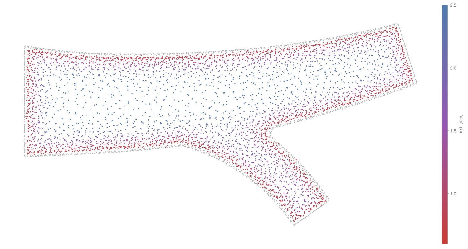
Interior cross-section of a vessel bifurcation filled with Orthtree + BoundaryLayerSpacing, each point colored by its local target spacing h(x) — red at the wall, blue in the bulk.

For a complete runnable script, see:

• examples/octree_boundary_layer.jl

SlakKosec

Default algorithm for 3D discretization. Generates candidate points on spheres around existing points, accepting those that are inside the domain and sufficiently far from existing points.

# Basic usage
cloud = discretize(boundary, spacing; alg=SlakKosec())

# Custom number of candidates per sphere (default: 10)
cloud = discretize(boundary, spacing; alg=SlakKosec(20))

# With octree acceleration for faster isinside queries
octree = TriangleOctree(import_mesh("model.stl", u"m"); min_ratio=1e-6)
cloud = discretize(boundary, spacing; alg=SlakKosec(octree))
cloud = discretize(boundary, spacing; alg=SlakKosec(20, octree))

Supports both ConstantSpacing and variable spacings (LogLike).

VanDerSandeFornberg

3D algorithm that projects a 2D grid onto the shadow plane and fills the volume layer by layer using sphere packing heights.

cloud = discretize(boundary, ConstantSpacing(1mm); alg=VanDerSandeFornberg())

Requires ConstantSpacing. Uses isinside (Green's function) for filtering generated points.

FornbergFlyer

2D-only algorithm. Uses a similar height-field approach as VanDerSandeFornberg, but projects onto the x-axis for 2D domains.

cloud = discretize(boundary, ConstantSpacing(0.1mm); alg=FornbergFlyer())

Must be requested explicitly — Orthtree is the 2D default, and the only 2D option for graded spacing.

Spacing Types

Spacing controls point density for all algorithms.

ConstantSpacing

Uniform spacing everywhere in the domain:

spacing = ConstantSpacing(1mm)

Works with all algorithms.

BoundaryLayerSpacing

Variable spacing specifically designed for boundary-layer refinement.

spacing = BoundaryLayerSpacing(
	points(boundary);
	at_wall=0.6m,
	bulk=4.0m,
	layer_thickness=8.0m,
)

• at_wall controls the smallest spacing near the boundary.

• bulk controls the largest spacing far from the boundary.

• layer_thickness sets how fast spacing transitions from wall to bulk.

boundary_points must be non-empty; distance queries are KDTree-accelerated. Works especially well with Orthtree.

LogLike

Variable spacing that is denser near the boundary and coarser in the interior. Uses a logarithmic-like growth function:

spacing = LogLike(cloud, base_size, growth_rate)

• cloud — An existing PointCloud. LogLike uses the cloud's boundary points to compute distances, so you must first create a cloud with ConstantSpacing, then use LogLike for a second-pass refinement.

• base_size — Spacing at the boundary surface.

• growth_rate — Rate at which spacing increases away from the boundary. Values > 1 create coarser interior points.

The spacing at a point is computed as base_size * x / (a + x) where x is the distance to the nearest boundary point.

Works with SlakKosec and Orthtree.

Typical workflow:

# First pass with uniform spacing
cloud = discretize(boundary, ConstantSpacing(1mm); alg=Orthtree(mesh))

# Second pass with variable spacing
spacing = LogLike(cloud, 0.5mm, 1.2)
cloud = discretize(boundary, spacing; alg=Orthtree(mesh))

References

• Slak, J. & Kosec, G. (2019). On generation of node distributions for meshless PDE discretizations. SIAM Journal on Scientific Computing, 41(5).

• Van der Sande, K. & Fornberg, B. (2021). Fast variable density 3-D node generation. SIAM Journal on Scientific Computing, 43(1).

• Fornberg, B. & Flyer, N. (2015). Fast generation of 2-D node distributions for mesh-free PDE discretizations. Computers & Mathematics with Applications, 69(7).