Vector & Tensor Operators

This guide demonstrates RBF-FD operators for vector calculus on scattered point clouds using the 2D Taylor-Green vortex — an incompressible flow with known analytical solutions for every quantity we compute.

For the operator type system, see Operators & Type Hierarchy. For basics, see Getting Started.

using RadialBasisFunctions
using StaticArrays
using CairoMakie
using Random

Setup: Taylor-Green Vortex

The Taylor-Green vortex is a classical test case in computational fluid dynamics. The velocity field on is:

This flow is incompressible (  ) and features counter-rotating vortices.

Random.seed!(42)

# Scattered points on [0, 2]² via jittered grid
n_side = 50
h = 2 / n_side
points = [
    SVector(
        clamp(h * (i - 0.5) + 0.3h * randn(), 0.01, 1.99),
        clamp(h * (j - 0.5) + 0.3h * randn(), 0.01, 1.99),
    ) for i in 1:n_side for j in 1:n_side
]

# Taylor-Green velocity field
u1 = [sin(π * p[1]) * cos(π * p[2]) for p in points]
u2 = [-cos(π * p[1]) * sin(π * p[2]) for p in points]
vel = hcat(u1, u2)

# Shared stencils for all operators
adjl = find_neighbors(points, 30)

# Visualization grid (inset to avoid boundary artifacts)
nx, ny = 80, 80
xs = range(0.05, 1.95; length=nx)
ys = range(0.05, 1.95; length=ny)
grid_points = vec([SVector(x, y) for x in xs, y in ys])
rg = regrid(points, grid_points)
to_grid(v) = reshape(rg(v), nx, ny)

We use regrid to project scattered results onto a regular grid for contour plots — a stencil-based interpolation that is itself an RBF-FD operator.

Velocity Field

speed = to_grid(sqrt.(u1 .^ 2 .+ u2 .^ 2))

# Subsample for arrows
idx = 1:8:length(points)
px = getindex.(points[idx], 1)
py = getindex.(points[idx], 2)

fig = Figure(; size=(600, 500))
ax = Axis(fig[1, 1]; xlabel="x", ylabel="y", title="Taylor-Green Velocity Field", aspect=1)
cf = contourf!(ax, xs, ys, speed; colormap=:viridis, levels=15)
arrows!(ax, px, py, 0.06 .* u1[idx], 0.06 .* u2[idx];
    color=:black, linewidth=0.8, arrowsize=6)
Colorbar(fig[1, 2], cf; label="Speed |u|")
fig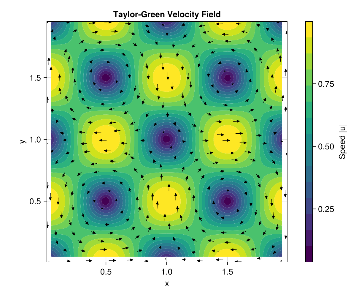

Divergence

The divergence measures local expansion or compression of a vector field:

For the Taylor-Green vortex,      — the flow is incompressible, so the numerical divergence should be near zero everywhere.

div_op = divergence(points; adjl=adjl)
div_u = div_op(vel)
println("Max |∇⋅u|: ", round(maximum(abs, div_u); sigdigits=3))

Max |∇⋅u|: 0.0383

div_grid = to_grid(div_u)
lim = maximum(abs, div_grid)

fig = Figure(; size=(600, 500))
ax = Axis(fig[1, 1]; xlabel="x", ylabel="y",
    title="Divergence ∇⋅u (incompressible → 0)", aspect=1)
cf = contourf!(ax, xs, ys, div_grid; colormap=:RdBu, levels=range(-lim, lim; length=20))
Colorbar(fig[1, 2], cf; label="∇⋅u")
fig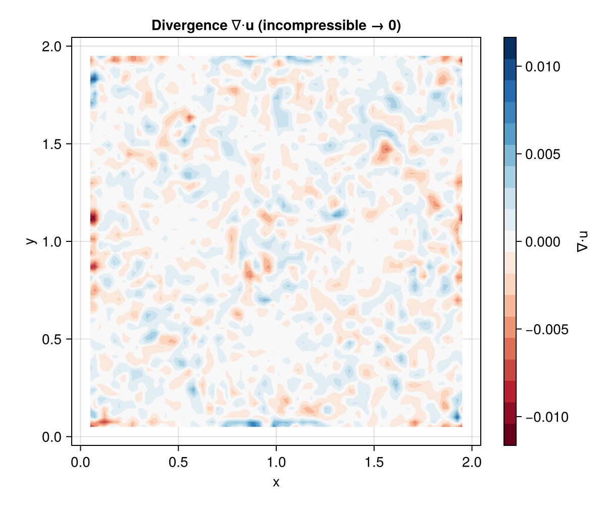

The symmetric pattern around zero confirms the flow is numerically incompressible — the small residuals are RBF-FD discretization error.

Curl (Vorticity)

In 2D, the curl reduces to a scalar — the vorticity:

curl_op = curl(points; adjl=adjl)
ω = curl_op(vel)

ω_exact = [2π * sin(π * p[1]) * sin(π * p[2]) for p in points]
println("Vorticity max error: ", round(maximum(abs, ω .- ω_exact); sigdigits=3))

Vorticity max error: 0.102

ω_grid = to_grid(ω)
ω_exact_grid = [2π * sin(π * x) * sin(π * y) for x in xs, y in ys]
lims = extrema(ω_exact_grid)
shared_levels = range(lims[1], lims[2]; length=20)

fig = Figure(; size=(900, 400))
ax1 = Axis(fig[1, 1]; xlabel="x", ylabel="y", title="RBF Vorticity", aspect=1)
contourf!(ax1, xs, ys, ω_grid; colormap=:RdBu, levels=shared_levels)

ax2 = Axis(fig[1, 2]; xlabel="x", ylabel="y", title="Analytical Vorticity", aspect=1)
cf = contourf!(ax2, xs, ys, ω_exact_grid; colormap=:RdBu, levels=shared_levels)

Colorbar(fig[1, 3], cf; label="ω")
fig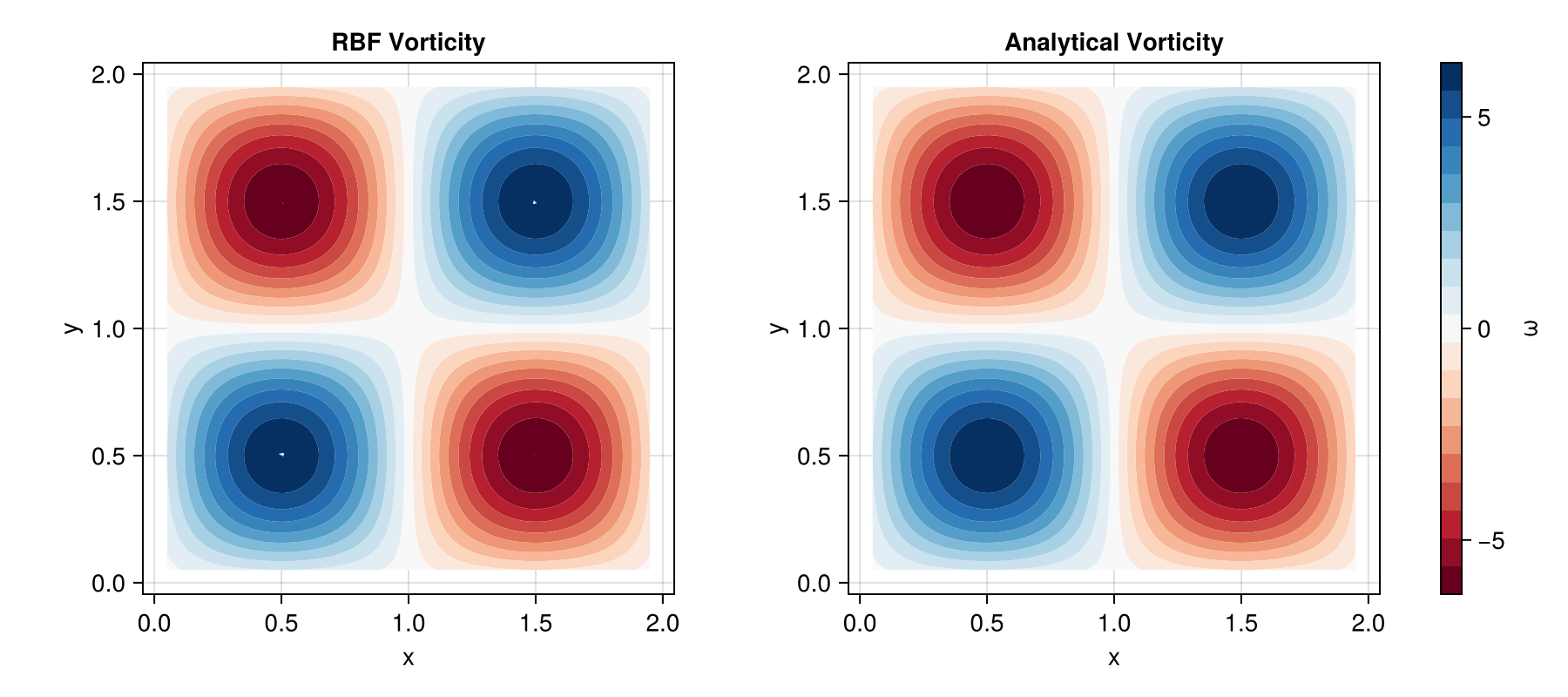

Jacobian (Velocity Gradient)

The Jacobian tensor contains all first-order partial derivatives of the velocity field:

The Jacobian is the building block for both the strain rate and rotation rate tensors.

jac_op = jacobian(points; adjl=adjl)
J = jac_op(vel)

J_exact = [
    [π * cos(π * p[1]) * cos(π * p[2]) for p in points],
    [-π * sin(π * p[1]) * sin(π * p[2]) for p in points],
    [π * sin(π * p[1]) * sin(π * p[2]) for p in points],
    [-π * cos(π * p[1]) * cos(π * p[2]) for p in points],
]

for (name, computed, exact) in zip(
    ["J₁₁", "J₁₂", "J₂₁", "J₂₂"],
    [J[:, 1, 1], J[:, 1, 2], J[:, 2, 1], J[:, 2, 2]],
    J_exact,
)
    println(name, " max error: ", round(maximum(abs, computed .- exact); sigdigits=3))
end

J₁₁ max error: 0.0331
J₁₂ max error: 0.0596
J₂₁ max error: 0.0443
J₂₂ max error: 0.0385

Strain Rate

The symmetric strain rate tensor measures the rate of deformation of fluid elements:

For the Taylor-Green vortex:  ,   , and the off-diagonal  .

ε_op = strain_rate(points; adjl=adjl)
ε = ε_op(vel)

ε11_exact = [π * cos(π * p[1]) * cos(π * p[2]) for p in points]
println("Symmetry check |ε₁₂ - ε₂₁|: ",
    round(maximum(abs, ε[:, 1, 2] .- ε[:, 2, 1]); sigdigits=3))
println("ε₁₁ max error: ", round(maximum(abs, ε[:, 1, 1] .- ε11_exact); sigdigits=3))
println("ε₁₂ max error (should be ≈ 0): ",
    round(maximum(abs, ε[:, 1, 2]); sigdigits=3))

Symmetry check |ε₁₂ - ε₂₁|: 0.0
ε₁₁ max error: 0.0331
ε₁₂ max error (should be ≈ 0): 0.0184

The strain rate magnitude   shows where the flow deforms fluid elements most strongly:

ε_mag = sqrt.(ε[:, 1, 1] .^ 2 .+ ε[:, 2, 2] .^ 2 .+ 2 .* ε[:, 1, 2] .^ 2)

fig = Figure(; size=(600, 500))
ax = Axis(fig[1, 1]; xlabel="x", ylabel="y",
    title="Strain Rate Magnitude ‖ε‖", aspect=1)
cf = contourf!(ax, xs, ys, to_grid(ε_mag); colormap=:inferno, levels=15)
Colorbar(fig[1, 2], cf; label="‖ε‖")
fig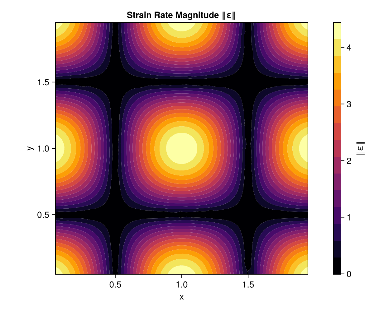

Rotation Rate

The antisymmetric rotation rate tensor captures local rigid-body rotation:

In 2D, the only independent component is   , where is the scalar vorticity from the curl.

Ω_op = rotation_rate(points; adjl=adjl)
Ω = Ω_op(vel)

println("Antisymmetry check |Ω₁₂ + Ω₂₁|: ",
    round(maximum(abs, Ω[:, 1, 2] .+ Ω[:, 2, 1]); sigdigits=3))
println("Identity check |Ω₁₂ + ½ω|: ",
    round(maximum(abs, Ω[:, 1, 2] .+ 0.5 .* ω); sigdigits=3))

Antisymmetry check |Ω₁₂ + Ω₂₁|: 0.0
Identity check |Ω₁₂ + ½ω|: 4.73e-14

The near-zero identity check confirms the fundamental relationship between the rotation rate tensor and scalar vorticity.

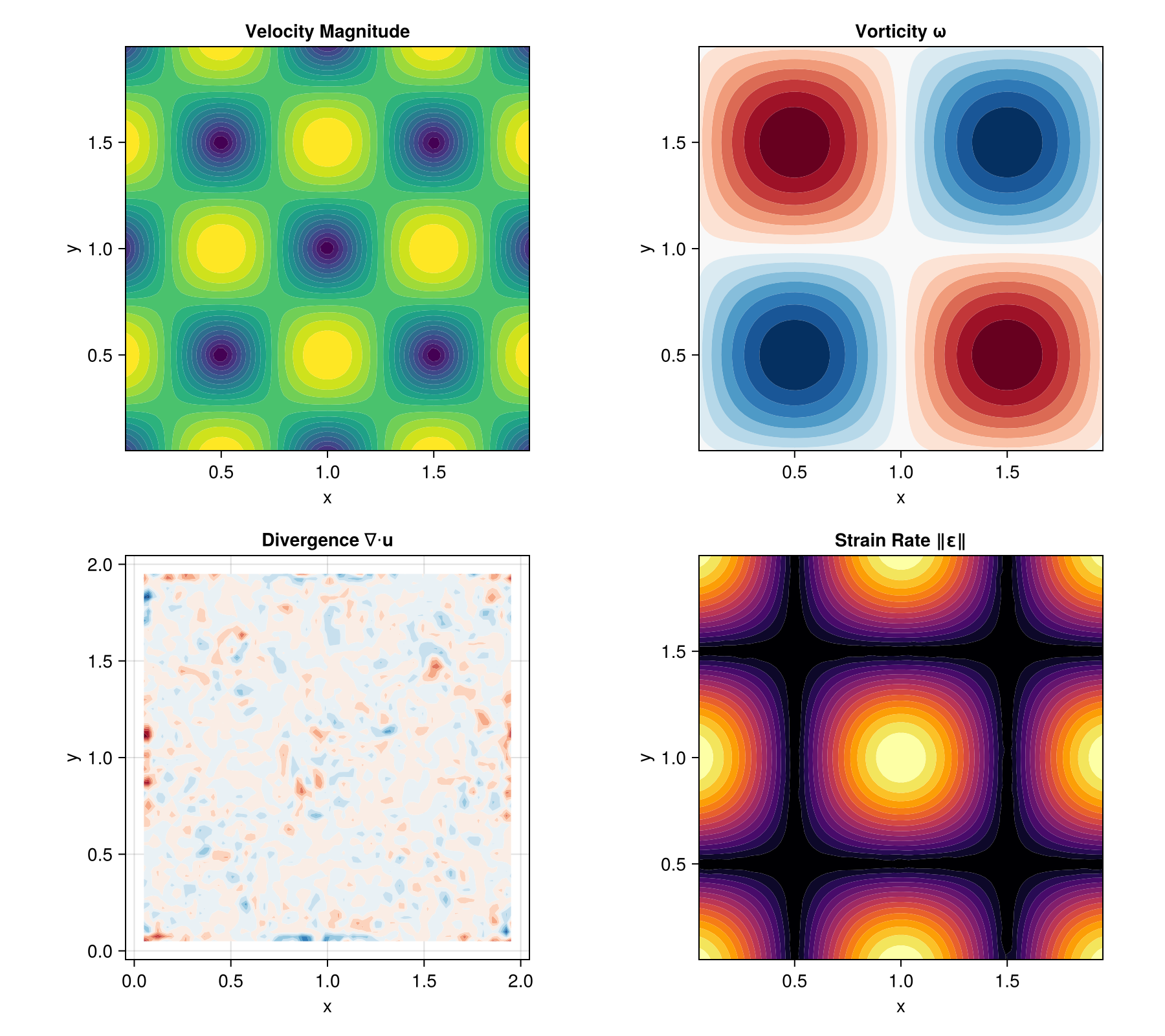
Summary

All five operators applied to the same scattered point cloud and velocity field:

fig = Figure(; size=(900, 800))

ax1 = Axis(fig[1, 1]; xlabel="x", ylabel="y", title="Velocity Magnitude", aspect=1)
contourf!(ax1, xs, ys, speed; colormap=:viridis, levels=15)

ax2 = Axis(fig[1, 2]; xlabel="x", ylabel="y", title="Vorticity ω", aspect=1)
contourf!(ax2, xs, ys, ω_grid; colormap=:RdBu, levels=15)

ax3 = Axis(fig[2, 1]; xlabel="x", ylabel="y", title="Divergence ∇⋅u", aspect=1)
contourf!(ax3, xs, ys, div_grid; colormap=:RdBu, levels=range(-lim, lim; length=15))

ax4 = Axis(fig[2, 2]; xlabel="x", ylabel="y", title="Strain Rate ‖ε‖", aspect=1)
contourf!(ax4, xs, ys, to_grid(ε_mag); colormap=:inferno, levels=15)

fig