Work-Precision

Convergence plots tell you which basis and polynomial degree are most accurate per point. Work-precision plots tell you what they cost. This page uses laplacian as a surrogate operator — the weight-assembly cost is nearly identical across local-stencil differential operators since they share the same local-system structure — and treats Interpolator separately because it uses a global stencil.

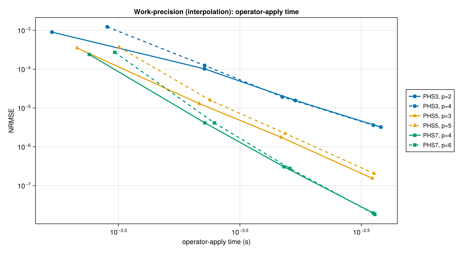
Each marker represents one (basis, poly_deg) configuration; connected markers are the same configuration at different N ∈ {225, 900, 2025, 4900}. The lower-left corner is "best": low error per unit time.

Plots below are PHS-only. Shape-parameter bases (IMQ, Gaussian) need ε scaled with stencil spacing to produce a fair cost comparison (see Shape-Parameter Bases for why); a cost study of the scaled-ε configs is not covered here.

Benchmark environment

Timings below were measured on: AMD Ryzen 9 9900X, 20 threads, Julia 1.12.6, RadialBasisFunctions 0.5.0. Absolute numbers will differ on other machines; the relative ordering of basis configurations is the informative part.

Weight build time — Laplacian

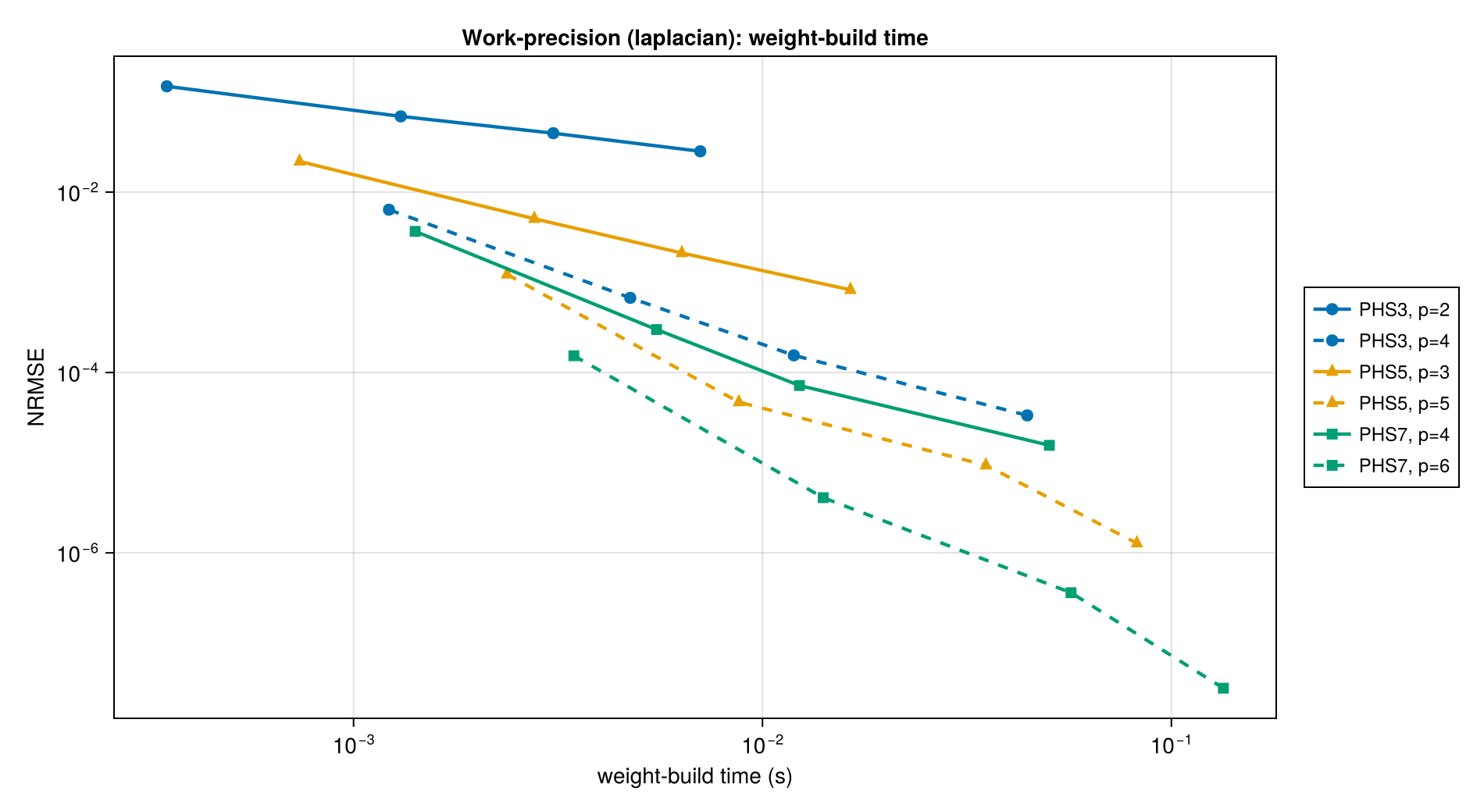
Each family appears twice: a solid curve at the matched polynomial degree (PHS3/p=2, PHS5/p=3, PHS7/p=4) and a dashed curve at a higher-poly_deg overshoot (p=4, p=5, p=6 respectively). The overshoot curves sit below their matched siblings — extra polynomial degree buys lower error at extra cost. Higher-order PHS dominates the Pareto frontier: PHS7/p=6 reaches the lowest error, PHS5/p=3 hits the sweet spot for most applications. PHS1/p=1 is omitted because its error is not useful for second-derivative operators (see the Laplacian section).

Apply time — Laplacian

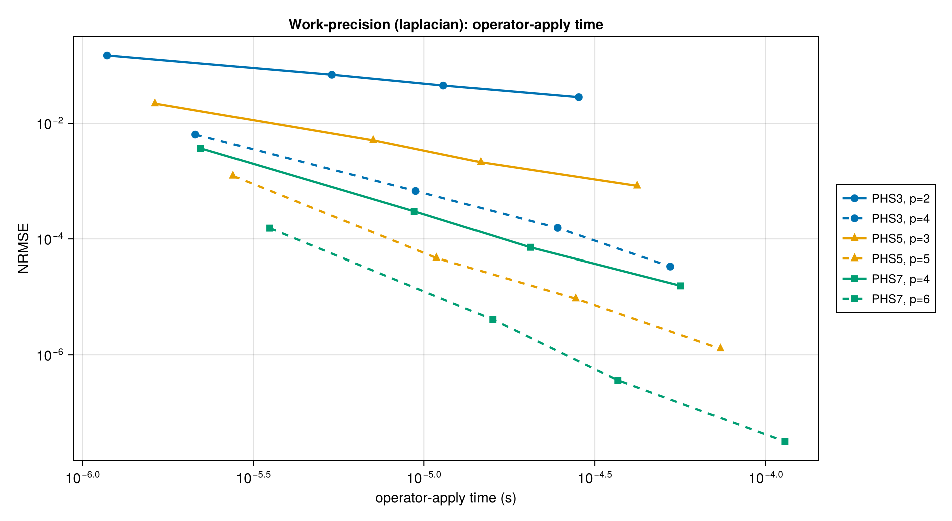
Apply time is 10–100× shorter than build time; once weights are built, applying the operator is a sparse matrix-vector product. This makes the "amortize over many applies" decision easy: if you apply the same operator many times (e.g., time-stepping a PDE), pick the highest-accuracy configuration you can afford during the one-time build.

Memory footprint — Laplacian

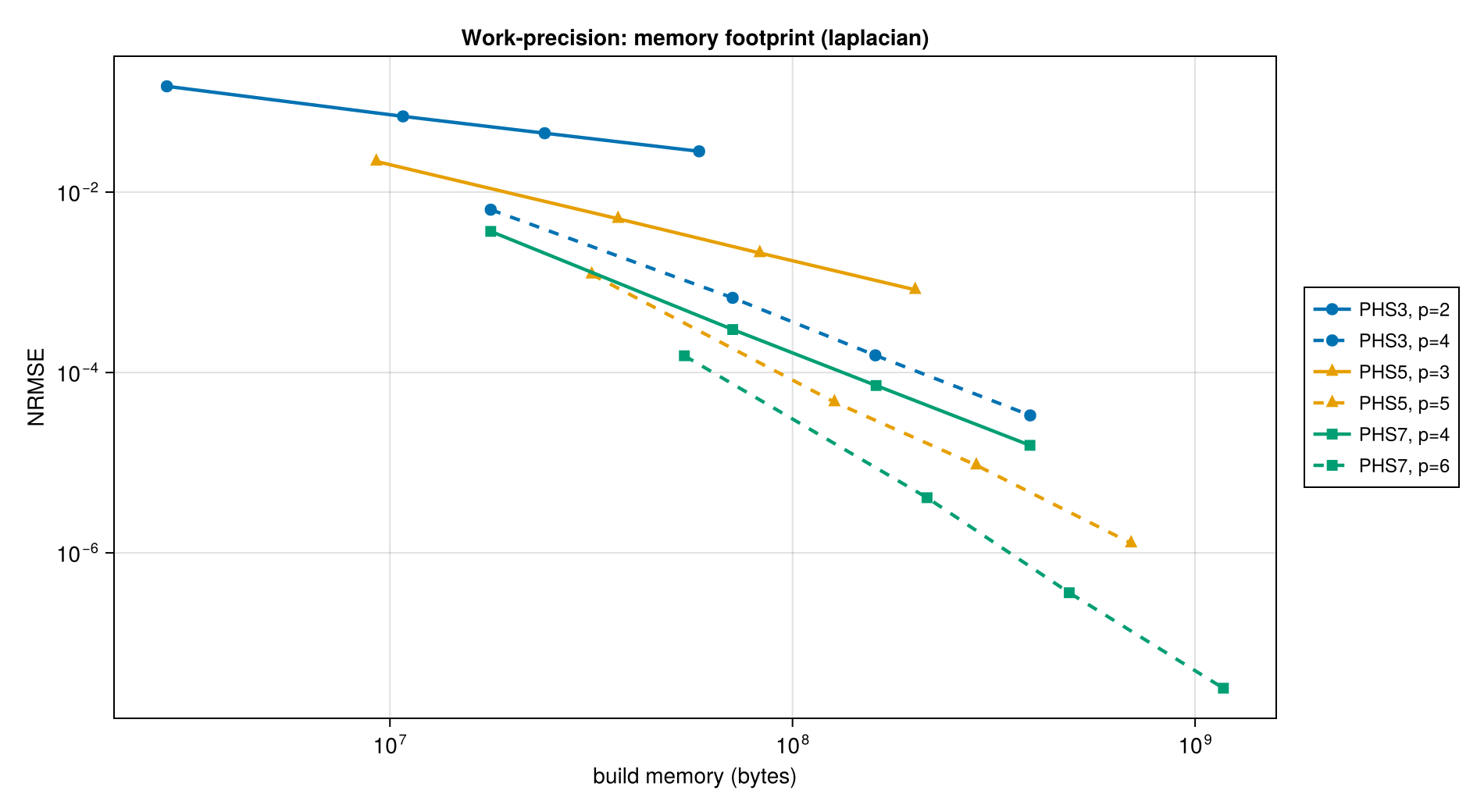
Memory scales with N × k × (k + npoly) — the local-system factorization cost. Higher poly_deg inflates both the stencil requirement and the factorization size.

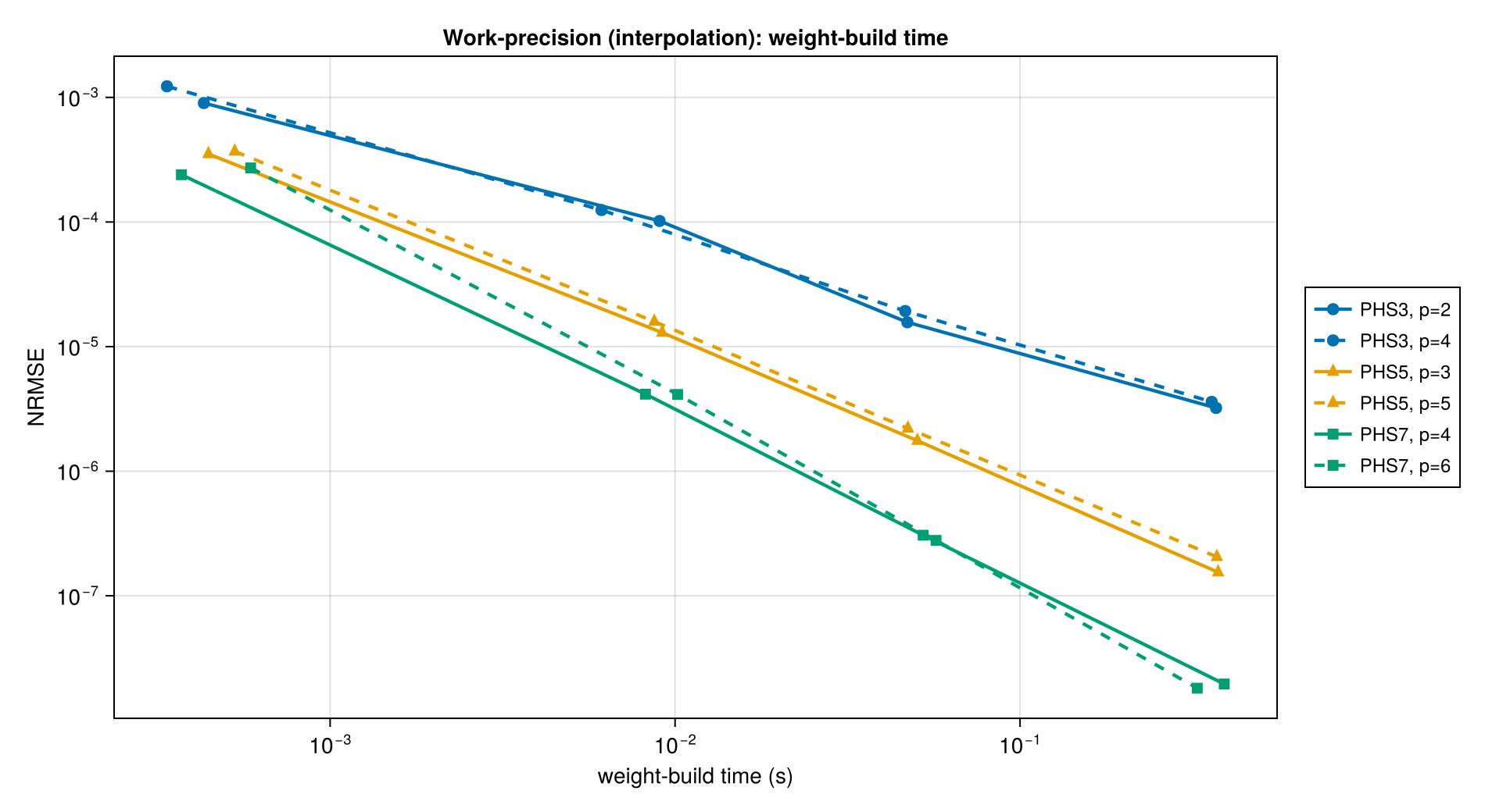
Interpolation

The Interpolator uses a global stencil: every evaluation touches every data point. Cost scales very differently from local-stencil operators — the build cost is dominated by a single N×N dense factorization, and the per-evaluation cost is O(N).

Build time

Apply time

For scattered-data interpolation over more than a few thousand points, this global approach becomes costly. Use regrid (local-stencil interpolation between point sets) when you need to transfer data at scale.

Practical guidance

• Default: PHS(3; poly_deg=2) — 2nd-order accurate, no tuning, well within 1 decade of the Pareto frontier on every plot above.

• When you need more accuracy: PHS(5; poly_deg=3) typically halves the error at ~3× the build cost. Beyond that, PHS7/p=4 offers diminishing returns unless you're targeting < 10⁻⁶ error.

• When build cost dominates: compute once, apply many times. The apply-time plot is roughly 10–100× faster than build.

• When you need mixed partials or the full Hessian: start at PHS5/p=3 regardless of cost — the matched PHS3/p=2 does not converge (see the scalar operators section).