Shape-Parameter Bases (IMQ, Gaussian)

Polyharmonic splines have no shape parameter and converge cleanly under h-refinement. The shape-parameter bases — IMQ and Gaussian — do not: their h-refinement behavior is dominated by the interaction between ε and the stencil spacing, and fixing ε across a refinement sweep causes observable error growth at large N. This page explains why and shows what cleans it up.

All IMQ / Gaussian h-refinement plots have been moved here so the operator pages can stay focused on rate / poly_deg comparisons.

The RBF uncertainty principle

For a stencil of physical radius h, the basis ϕ(r) = exp(-(εr)²) (Gaussian) or ϕ(r) = 1/√(1+(εr)²) (IMQ) is characterized entirely by the non-dimensional product ε·h. Two limits:

• ε·h → ∞ (peaked basis, large ε relative to spacing): the RBF decays to zero between neighbors. The local system approaches a diagonal interpolant with poor approximation power.

• ε·h → 0 (flat basis, small ε relative to spacing): every RBF evaluates to nearly the same value across the stencil. The RBF columns of the collocation matrix lose linear independence, the system is ill-conditioned, and the solved stencil weights grow large with alternating signs. Multiplying those weights through the evaluation amplifies floating-point roundoff error.

Truncation error (analytic approximation error) shrinks as ε·h → 0, but rounding error grows. The two cross over at a problem-specific sweet spot — the trade-off principle of Schaback [1], revisited by Driscoll & Fornberg [2] and Fornberg & Flyer [3]. An ε-refinement sweep at fixed N shows this directly as a U-shape in NRMSE vs ε (see data/eps_refinement.csv).

Now consider h-refinement with ε held constant. Stencil size k is fixed per configuration, so as N grows the physical stencil radius shrinks as h ~ 1/√N. The product ε·h collapses toward zero, driving the system into the ill-conditioned regime. Error first decreases (truncation dominates), then bottoms out and rises (rounding dominates). This is the "fixed ε" story below.

PHS is immune: it has no shape parameter and is scale-invariant when paired with polynomial augmentation, so stencil shrinkage doesn't change conditioning.

Fixed ε = 1 vs scaled ε = c/h

The fix is to scale ε so that ε·h stays near the sweet spot as N grows. Stationary scaling ε = c/h keeps the non-dimensional basis shape constant across the sweep. The constants c below are calibrated from the fixed-N ε-refinement minima in eps_refinement.csv at N=900:

Operator	c	Rationale
Interpolation	0.15	ε_opt ≈ 3–6 at h = 1/30 → ε·h ≈ 0.10–0.21
Laplacian	0.03	ε_opt ≈ 0.5–1.0 → ε·h ≈ 0.017–0.033
Mixed partial	0.03	Same order (2nd derivative), same scaling

Each plot below shows the same operator twice:

• Left: IMQ and Gaussian with ε = 1 — the standard curves from the h_refinement.csv sweep, reproduced here.

• Right: IMQ and Gaussian with ε = c/h — a new sweep (hseps target in generate_data.jl) that holds ε·h constant.

A PHS5/p=3 curve from the matched-degree sweep appears on both panels as a non-shape-parameter reference. The y-axis is shared across panels.

Interpolation

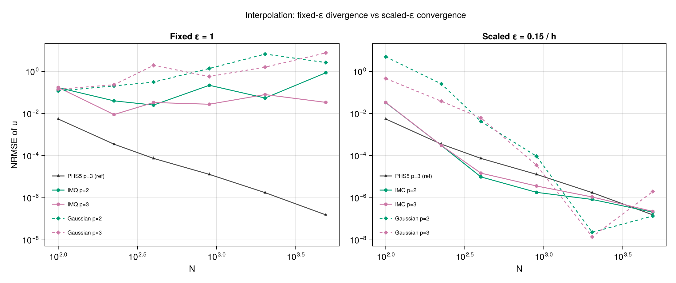
The fixed-ε panel shows non-monotone behavior and poly_deg-dependent stagnation. Scaled ε recovers clean convergence; at large N the shape-parameter bases beat the PHS5/p=3 reference by one to two orders of magnitude because a well- tuned Gaussian or IMQ approaches spectral accuracy on smooth targets.

Laplacian

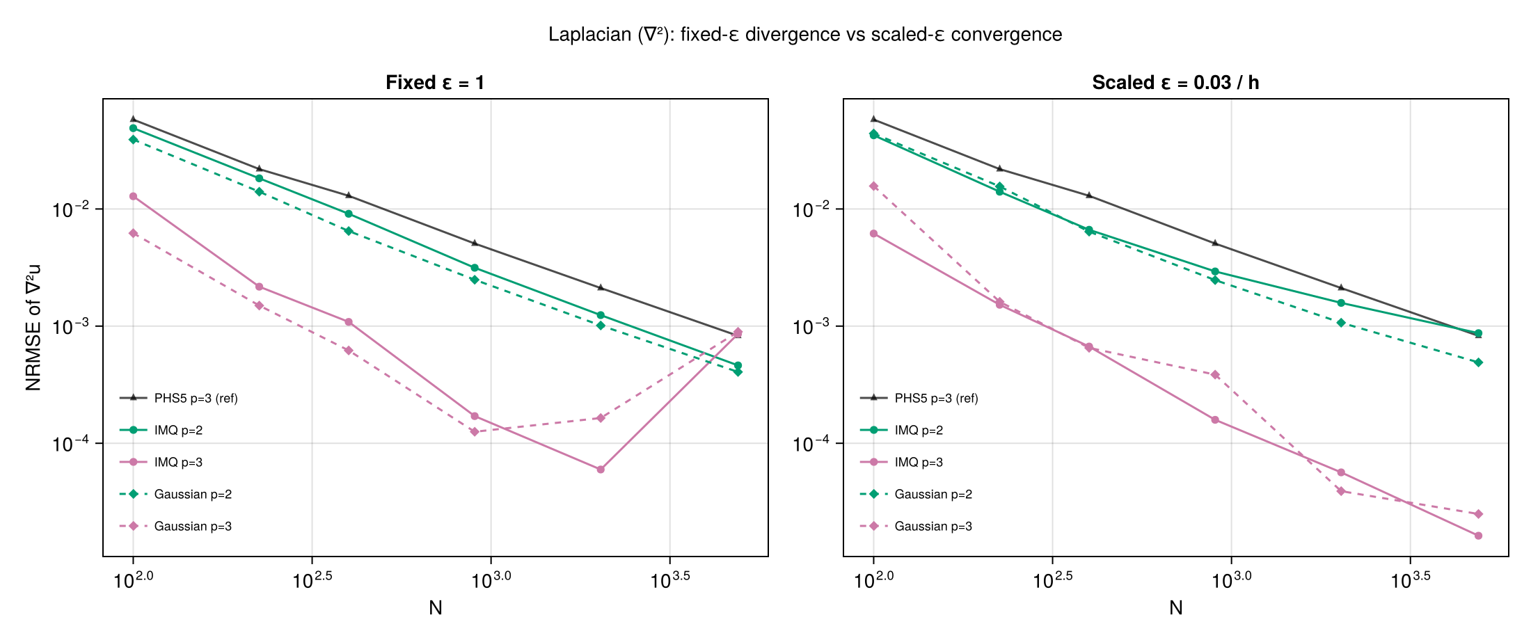
At ε = 1 the p=2 curves flatten or turn up past N ≈ 2000; scaled ε restores steady ~O(h²)–O(h³) convergence, with p=3 matching or beating PHS5/p=3.

Mixed partial

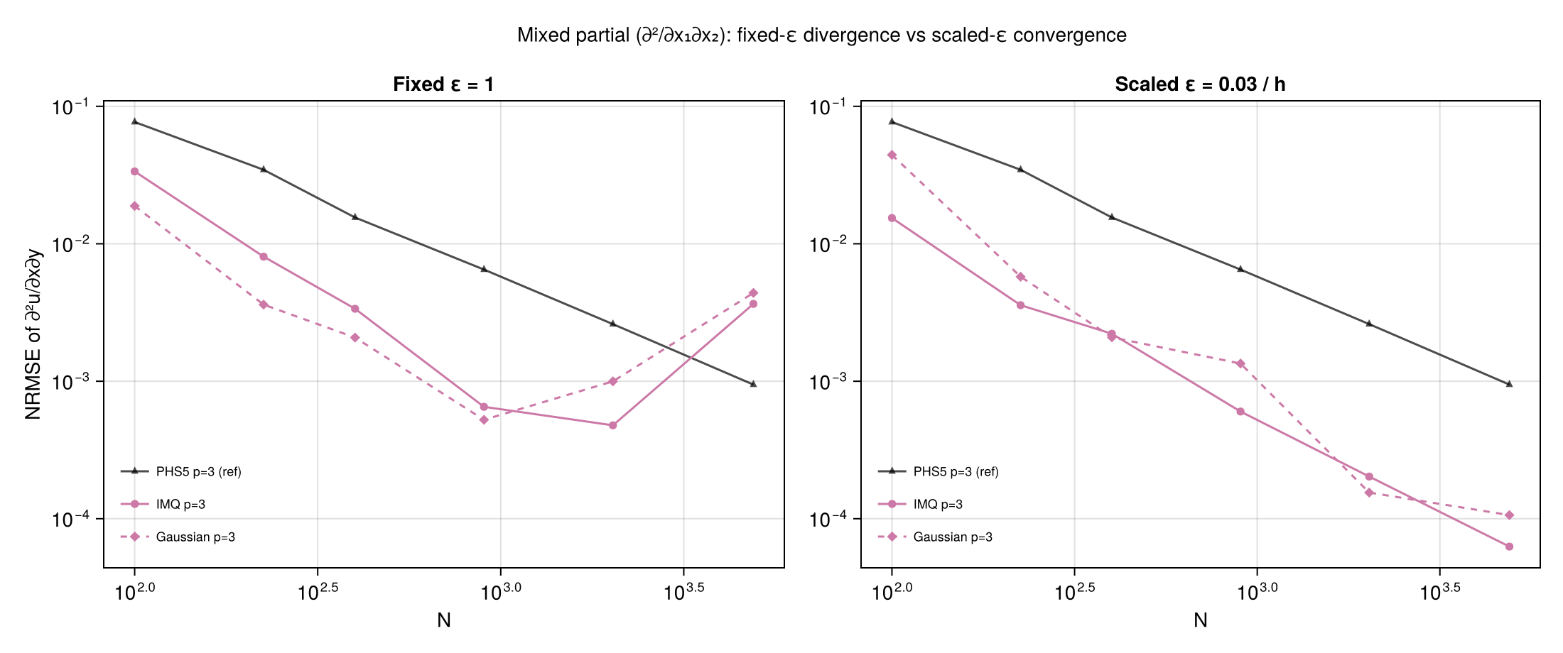
Only p=3 is shown — p=0 and p=2 don't converge for mixed partials with shape-parameter bases regardless of ε (a polynomial-augmentation issue, not a conditioning one — see the mixed partial section). With p=3, fixed ε shows the classic turnaround around N ≈ 2000; scaled ε converges cleanly.

Practical guidance

• PHS is the default. No parameter tuning, no conditioning cliff. Use PHS(3; poly_deg=2) or PHS(5; poly_deg=3) unless a specific reason motivates shape-parameter bases.

• If you use IMQ or Gaussian: scale ε with the local stencil spacing. For a quasi-uniform point cloud, ε ≈ c / h with c calibrated once via an ε-refinement sweep at representative N is straightforward. Do not carry a single ε across problems of different resolution without retuning.

• Stable evaluation. Algorithms like RBF-QR [4] and Contour–Padé [5] compute stable weights across the full ε range without the uncertainty principle, but are not currently implemented in this package.

References

1. Schaback, R. (1995). Error estimates and condition numbers for radial basis function interpolation. Advances in Computational Mathematics, 3, 251–264. DOI: 10.1007/BF02432002. Original formulation of the trade-off / uncertainty principle.

2. Driscoll, T. A. and Fornberg, B. (2002). Interpolation in the limit of increasingly flat radial basis functions. Computers & Mathematics with Applications, 43(3–5), 413–422. DOI: 10.1016/S0898-1221(01)00295-4.

3. Fornberg, B. and Flyer, N. (2015). A Primer on Radial Basis Functions with Applications to the Geosciences. CBMS-NSF Regional Conference Series in Applied Mathematics, SIAM. Chapter 4 covers the conditioning–accuracy trade-off in detail.

4. Fornberg, B. and Wright, G. (2004). Stable computation of multiquadric interpolants for all values of the shape parameter. Computers & Mathematics with Applications, 48(5–6), 853–867. DOI: 10.1016/j.camwa.2003.08.010.

5. Fornberg, B., Larsson, E., and Wright, G. (2004). A new class of oscillatory radial basis functions. Computers & Mathematics with Applications, 51(8), 1209–1222. DOI: 10.1016/j.camwa.2006.04.004.