RBF Neural Networks

Radial basis functions aren't just for meshfree PDE methods — they make excellent neural network activation functions. This page covers the theory behind RBF networks and walks through a hands-on comparison with a standard MLP using Lux.jl.

Why RBF Activations?

Local vs Global Activations

Standard activations like ReLU, tanh, and sigmoid are global: they partition the entire input space with hyperplanes, so every neuron responds to every input. Radial basis functions are local: each neuron is centered at a point in input space and responds most strongly to inputs near that center, decaying smoothly with distance.

This locality is particularly valuable for physics-informed neural networks (PINNs). Shouwei Li et al. (2024) introduced PIRBN (Physics-Informed Radial Basis Networks) and showed that PINNs naturally drift toward local approximation during training — RBF activations align with this tendency rather than fighting it, leading to faster convergence and better accuracy on PDEs.

The KAN–RBF Equivalence

Kolmogorov–Arnold Networks (KANs) attracted significant attention for placing learnable activation functions on edges rather than nodes. Li (2024) proved that KANs with RBF activations are mathematically equivalent to RBF networks, and that the simpler RBF formulation is faster in practice:

Model	Test RMSE (function approx.)	Training time
Original KAN (B-spline)	Baseline	Baseline
FastKAN (Gaussian RBF)	Comparable	3.3× faster
RBF-KAN (equivalence)	Comparable	Faster than KAN

More recently, Putri et al. (2026) proved universal approximation for Free-RBF-KAN architectures with learnable centers, widths, and weights — confirming that RBF networks have the same expressive power as KANs without the implementation complexity.

Advantages for Scientific Computing

RBF activations inherit mathematical properties that standard activations lack:

Property	RBF layer	Dense + ReLU/tanh
Smoothness	(Gaussian, IMQ)	(ReLU), (tanh)
Locality	Each neuron covers a region	Every neuron responds globally
Interpolation guarantee	Exact with enough centers	No guarantee
Polynomial reproduction	Built-in via augmentation	Learned only
Known convergence rates	Yes (scattered data theory)	No
Interpretable parameters	Centers, shape params	Opaque weights

Where RBF Layers Excel

RBF activations show the largest gains in scientific and geometric computing tasks:

Application	Key result	Reference
PDE solving (PINNs)	1000× better error vs standard PINNs	RBF-PINN (Wang et al., 2024)
Physics-informed networks	Faster convergence on Poisson, Helmholtz, Burgers	PIRBN (Li et al., 2024)
Neural radiance fields	10–100× fewer parameters for same quality	NeuRBF (Chen et al., 2023)
Neural fields (geometry)	Compact representation of SDFs and textures	NeuRBF (Chen et al., 2023)
Function approximation	Matches KAN accuracy, simpler architecture	FastKAN / RBF-KAN (Li, 2024)

Learnable Shape Parameters

The shape parameter controls how wide or narrow each basis function is. Rather than fixing it, RBFLayer makes a learnable parameter trained end-to-end via gradient descent.

Internally, the layer stores an unconstrained parameter and maps it through softplus to guarantee positivity:

Initialization matters. Starting with too large (narrow peaks) makes gradients vanish; too small (flat plateaus) makes all centers indistinguishable. The default initialization scales inversely with the number of centers, placing the network in a regime where basis functions overlap enough for smooth gradients but are distinct enough to specialize during training.

Training an RBF Network

This section trains an RBF network and a standard MLP on the same 1-D regression problem so you can compare convergence, accuracy, and interpretability.

Setup

using RadialBasisFunctions
using Lux, Optimisers, DifferentiationInterface, Mooncake
using Random, Statistics
using CairoMakie

const RBFLayer = Base.get_extension(
    RadialBasisFunctions, :RadialBasisFunctionsLuxCoreExt
).RBFLayer

rng = Random.MersenneTwister(0)

# Target function with low- and high-frequency components
f(x) = sin(3x) + 0.3f0 * cos(7x)

# Training data: 50 points on [-1, 1]
n_train = 50
x_train = collect(Float32, range(-1, 1; length=n_train))
y_train = f.(x_train)

# Dense evaluation grid for plotting
x_plot = collect(Float32, range(-1, 1; length=300))
y_true = f.(x_plot)

Model Definitions

Both models use roughly the same number of parameters so the comparison is fair.

# RBF network: 20 Gaussian centers
rbf_model = Chain(RBFLayer(1, 20, 1; basis_type=Gaussian))

# MLP: single hidden layer with relu activation
mlp_model = Chain(Dense(1 => 20, relu), Dense(20 => 1))

# Initialize
ps_rbf, st_rbf = Lux.setup(rng, rbf_model)
ps_mlp, st_mlp = Lux.setup(rng, mlp_model)

println("RBF parameters: ", Lux.parameterlength(rbf_model))
println("MLP parameters: ", Lux.parameterlength(mlp_model))

RBF parameters: 61
MLP parameters: 61

Training

A shared training loop keeps things comparable. Both models are trained with Adam for 1000 epochs on MSE loss.

function train(model, ps, st; lr=0.01f0, epochs=1000)
    ps_flat, restructure = Optimisers.destructure(ps)
    opt_state = Optimisers.setup(Adam(lr), ps_flat)
    X = reshape(x_train, 1, :)
    Y = reshape(y_train, 1, :)
    backend = AutoMooncake(; config=nothing)
    loss_fn(p) = mean((first(model(X, restructure(p), st)) .- Y) .^ 2)
    losses = Float32[]
    for epoch in 1:epochs
        val, grads = DifferentiationInterface.value_and_gradient(loss_fn, backend, ps_flat)
        push!(losses, val)
        opt_state, ps_flat = Optimisers.update(opt_state, ps_flat, grads)
    end
    return restructure(ps_flat), losses
end

ps_rbf_trained, losses_rbf = train(rbf_model, ps_rbf, st_rbf)
ps_mlp_trained, losses_mlp = train(mlp_model, ps_mlp, st_mlp)

println("RBF  final MSE: ", round(losses_rbf[end]; sigdigits=3))
println("MLP  final MSE: ", round(losses_mlp[end]; sigdigits=3))

RBF  final MSE: 0.000338
MLP  final MSE: 0.000911

Loss Curves

fig = Figure(; size=(600, 350));
ax = Makie.Axis(fig[1, 1];
    xlabel="Epoch", ylabel="MSE (log scale)",
    yscale=log10, title="Training convergence")
lines!(ax, losses_rbf; label="RBF", linewidth=2)
lines!(ax, losses_mlp; label="MLP", linewidth=2, linestyle=:dash)
axislegend(ax; position=:rt)
fig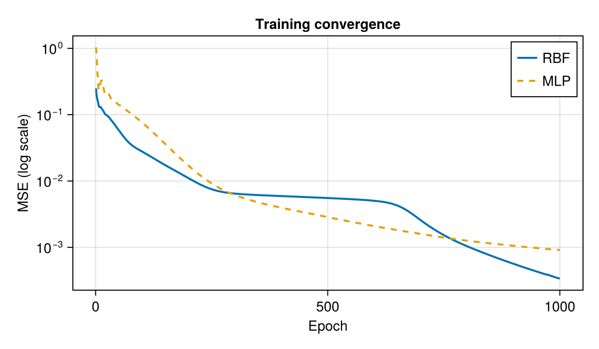

Final Fit

X_plot = reshape(x_plot, 1, :)
y_rbf, _ = rbf_model(X_plot, ps_rbf_trained, st_rbf)
y_mlp, _ = mlp_model(X_plot, ps_mlp_trained, st_mlp)

fig = Figure(; size=(700, 400));
ax = Makie.Axis(fig[1, 1]; xlabel="x", ylabel="f(x)", title="Learned fits after 1000 epochs")
lines!(ax, x_plot, y_true; label="Target", color=:black, linewidth=2)
lines!(ax, x_plot, vec(y_rbf); label="RBF", linewidth=2)
lines!(ax, x_plot, vec(y_mlp); label="MLP", linewidth=2, linestyle=:dash)
scatter!(ax, x_train, y_train; label="Training data", markersize=5, color=:gray)
axislegend(ax; position=:lb)
fig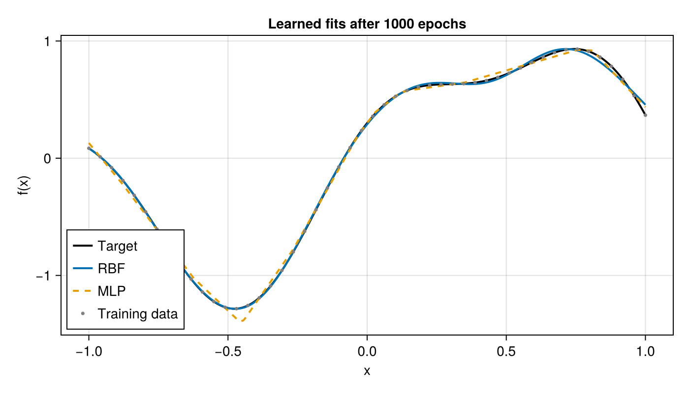

Learned Centers

A unique advantage of RBFLayer is that the centers are interpretable — each one anchors a basis function at a specific location in the input space.

centers = vec(ps_rbf_trained.layer_1.centers)

fig = Figure(; size=(700, 350));
ax = Makie.Axis(fig[1, 1]; xlabel="x", ylabel="f(x)", title="Learned RBF center locations")
lines!(ax, x_plot, y_true; color=:black, linewidth=2, label="Target")
vlines!(ax, centers; color=(:red, 0.5), linewidth=1.5, label="Centers")
axislegend(ax; position=:lb)
fig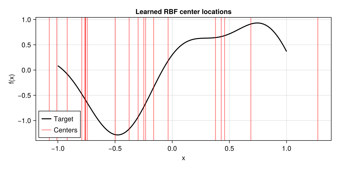

When to Use Standard Activations Instead

RBF layers are not universally superior. Prefer standard Dense + activation when:

• High-dimensional, non-spatial inputs — Euclidean distance becomes less meaningful beyond ~10–20 dimensions (curse of dimensionality). Tabular data with mixed categorical/numerical features is better served by ReLU networks.

• Deep architectures — Stacking many RBF layers is less studied than deep ReLU/transformer networks. For tasks requiring depth (NLP, large-scale vision), standard architectures have more mature tooling and theory.

• Massive scale — When training on millions of samples with thousands of features, the per-neuron distance computation in RBF layers adds overhead compared to a simple matrix multiply + pointwise activation.

• No geometric structure — If inputs have no notion of "closeness" (e.g., one-hot encoded categories, graph node IDs), locality provides no benefit.

References

1. S. Li, Y. Liu, & L. Liu, "PIRBN: Physics-Informed Radial Basis Networks," arXiv:2404.01445, 2024. Link

2. Z. Li, "Kolmogorov–Arnold Networks are Radial Basis Function Networks," arXiv:2405.06721, 2024. Link

3. J. Zhu, "FastKAN: Very Fast Kolmogorov-Arnold Networks," GitHub, 2024. Link

4. D. A. Putri, A. P. Tirtawardhana, & J. H. Yong, "Free-RBF-KAN," Engineering Applications of Artificial Intelligence, 2026. Link

5. Z. Wang, W. Xing, R. Kirby, & S. Zhe, "RBF-PINN: Non-Fourier Positional Embedding in Physics-Informed Neural Networks," arXiv:2402.08367, 2024. Link

6. Z. Chen, T. Li, Z. Ding, C. Wang, H. Bao, & Z. Chen, "NeuRBF: A Neural Fields Representation with Adaptive Radial Basis Functions," ICCV, 2023. Link