Getting Started

This tutorial walks through a complete 2D steady-state heat conduction simulation — from geometry to results. Along the way, it explains the key types and how they compose.

Installation

using Pkg
Pkg.add(url="https://github.com/JuliaMeshless/WhatsThePoint.jl")
Pkg.add(url="https://github.com/JuliaMeshless/RadialBasisFunctions.jl")
Pkg.add(url="https://github.com/JuliaMeshless/Macchiato.jl")

Step 1: Define the Geometry

Every simulation starts with a point cloud — a set of scattered points that discretize the domain boundary and interior. WhatsThePoint.jl handles this.

using WhatsThePoint
using Unitful: m, °

# Create a 1m × 1m rectangle boundary with points and normals
part = PointBoundary(rectangle(1m, 1m)...)

# Split the continuous boundary into 4 named surfaces at 75° corners
split_surface!(part, 75°)
# This creates :surface1 (bottom), :surface2 (right), :surface3 (top), :surface4 (left)

PointBoundary{Meshes.𝔼{2}, CoordRefSystems.Cartesian2D{CoordRefSystems.NoDatum, Unitful.Quantity{Float64, 𝐋, Unitful.FreeUnits{(m,), 𝐋, nothing}}}}
├─396 points
└─Surfaces
  ├─surface1
  ├─surface2
  ├─surface3
  └─surface4

Splitting at corners creates named surfaces so you can assign different boundary conditions to each edge. Now fill the interior:

# Discretize: place interior points at ~1/33 m spacing
dx = 1/33 * m
cloud = discretize(part, ConstantSpacing(dx), alg=VanDerSandeFornberg())

PointCloud{Meshes.𝔼{2}, CoordRefSystems.Cartesian2D{CoordRefSystems.NoDatum, Unitful.Quantity{Float64, 𝐋, Unitful.FreeUnits{(m,), 𝐋, nothing}}}}
├─1552 points
├─Boundary: 396 points
│ ├─surface1
│ ├─surface2
│ ├─surface3
│ └─surface4
├─Volume: 1156 points
└─Topology: NoTopology

The resulting PointCloud contains both boundary points (organized by surface) and interior (volume) points.

Step 2: Define the Physics Model

Physics models define the PDE being solved. For heat conduction, use SolidEnergy:

using Macchiato

model = SolidEnergy(k=1.0, ρ=1.0, cₚ=1.0)

Energy: (k = 1.0, ρ = 1.0, cₚ = 1.0)

This defines the heat equation with thermal conductivity k, density ρ, and specific heat cₚ.

Solving your own PDE?

SolidEnergy is one of several built-in models, but you can define a model for any PDE. See the Custom PDEs tutorial to learn how.

Step 3: Define Boundary Conditions

Boundary conditions are specified as a Dict mapping surface names to BC objects:

bcs = Dict(
    :surface1 => Temperature(0.0),    # bottom: T = 0
    :surface2 => Temperature(0.0),    # right:  T = 0
    :surface3 => Temperature(100.0),  # top:    T = 100
    :surface4 => Temperature(0.0)     # left:   T = 0
)

Dict{Symbol, PrescribedValue{Macchiato.var"#Temperature##0#Temperature##1"{Float64}}} with 4 entries:
  :surface4 => Temperature
  :surface3 => Temperature
  :surface2 => Temperature
  :surface1 => Temperature

Temperature is a Dirichlet BC — it prescribes the value directly. The BC system is organized by mathematical type:

Type	Meaning	Energy Examples
Dirichlet	Prescribes value: `u = g`	`Temperature`
Neumann	Prescribes flux: `∂u/∂n = q`	`HeatFlux`, `Adiabatic`
Robin	Mixed: `α u + β ∂u/∂n = g`	`Convection`

All BCs accept either a constant value or a function (x, t) -> value for spatially or temporally varying conditions:

# Spatially varying temperature
Temperature((x, t) -> 100.0 * sin(π * x[1]))

# Insulated boundary (zero heat flux)
Adiabatic()

# Convective cooling: h=10, k=1, T_ambient=25
Convection(10.0, 1.0, 25.0)

See the API Reference for the complete list of boundary condition types.

Named BCs are aliases for generic types

Temperature, HeatFlux, and Adiabatic are constructor functions that create PrescribedValue, PrescribedFlux, and ZeroFlux instances with a physics-meaningful display name. When defining a custom PDE, you can use the generic constructors directly — PrescribedValue(0.0), PrescribedFlux(1.0), ZeroFlux() — with no trait boilerplate required.

Step 4: Create the Domain

The Domain ties geometry, boundary conditions, and model together:

domain = Domain(cloud, bcs, model)

domain1: DomainSolidEnergy{Float64, Float64, Float64, Nothing}[Energy: (k = 1.0, ρ = 1.0, cₚ = 1.0)]

The Domain validates that every BC key matches a surface in the point cloud.

Step 5: Create and Run the Simulation

sim = Simulation(domain)
run!(sim)

Simulation
├── Mode: Steady-state
├── Time: 0.0
└── Running: false

Simulation defaults to steady-state when no mode is given:

Steady() (default) — assembles Ax = b and solves with LinearSolve.jl
Transient(Δt=..., stop_time=...) — builds an ODE right-hand side and integrates with OrdinaryDiffEq.jl

For steady-state, run! calls LinearSolve.LinearProblem(domain) internally, which:

Asks the model to build its system matrix and RHS via make_system
Applies each BC by modifying the appropriate matrix rows
Solves the sparse linear system

Step 6: Extract and Visualize Results

using WhatsThePoint: coords
using Unitful: ustrip
using CairoMakie

# Extract the temperature field
T = temperature(sim)

# Visualize the temperature field
pts = points(cloud)
x = [ustrip(coords(pt).x) for pt in pts]
y = [ustrip(coords(pt).y) for pt in pts]

fig = Figure(; size=(800, 700))
ax = Axis(fig[1, 1]; title="Temperature", xlabel="x [m]", ylabel="y [m]", aspect=DataAspect())
sc = scatter!(ax, x, y; color=T, colormap=:inferno, markersize=8)
Colorbar(fig[1, 2], sc; label="T")
fig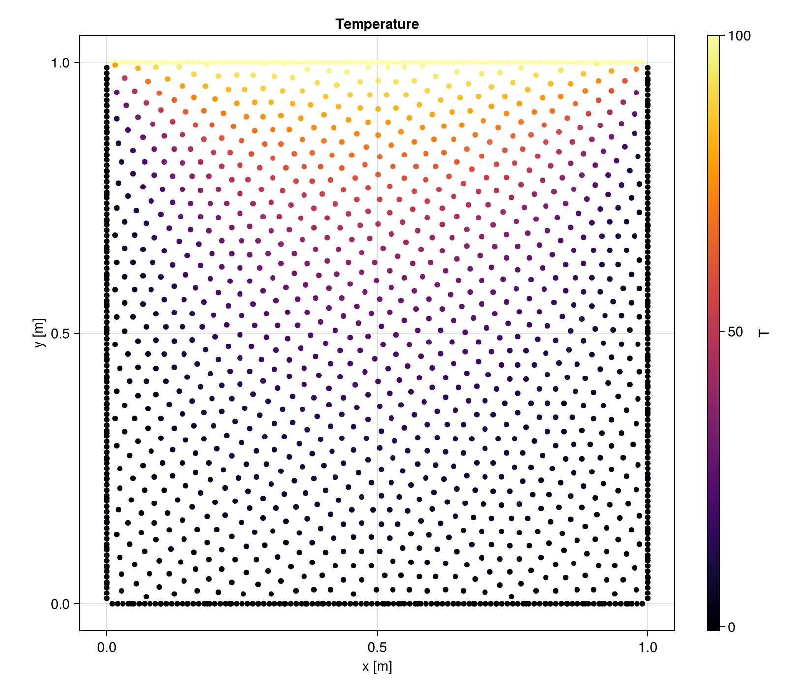

Each physics model has dedicated field extraction functions:

temperature(sim) — for SolidEnergy
displacement(sim) — for LinearElasticity, returns (ux, uy) or (ux, uy, uz)
velocity(sim), pressure(sim) — for IncompressibleNavierStokes

Going Transient

Converting the same problem to a transient simulation requires minimal changes — add a time step and stop time, and set initial conditions:

# Same domain as before
sim = Simulation(domain, Transient(Δt=0.001, stop_time=1.0))

# Set initial temperature to 0 everywhere
set!(sim, T=0.0)

# Or use a function of position
set!(sim, T=x -> 50.0 * exp(-10 * ((x[1]-0.5)^2 + (x[2]-0.5)^2)))

# Run transient simulation (time-steps with Tsit5 by default)
run!(sim)

T_final = temperature(sim)

1552-element Vector{Float64}:
  0.13683533716074592
  0.15077343572848984
  0.16579934371661179
  0.1819584354615585
  0.19929343460639307
  0.21784379830107542
  0.2376450762638495
  0.2587282503453219
  0.2811190610526966
  0.30483732827571025
  ⋮
 63.38976917719544
 57.940069146394855
 60.23390515748731
 63.58075025512214
 49.904799968389064
 62.715875225357834
 61.76764342084232
 64.03468481374827
 63.865505892260444